Tutorials
This section will guide you in the Mirheo interface step by step with examples.
Hello World: run Mirheo
We start with a very minimal script running Mirheo.
#!/usr/bin/env python

# first we need to import the module
import mirheo as mir

dt = 0.001                  # simulation time step
ranks  = (1, 1, 1)          # number of ranks in x, y, z directions
domain = (32.0, 16.0, 16.0) # domain size in x, y, z directions

# create the coordinator
u = mir.Mirheo(ranks, domain, debug_level=3, log_filename='log')

u.run(100, dt=dt) # Run 100 time-steps
The time step of the simulation and the domain size are common to all objects in the simulation,
hence it has to be passed to the coordinator (see its constructor).
We do not add anything more before running the simulation (last line).
Note
We also specified the number of ranks in each direction. Together with the domain size, this tells Mirheo how the simulation domain will be split across MPI ranks. The number of simulation tasks must correspond to this variable.
The above script can be run as:
mpirun -np 1 python3 hello.py
Running hello.py will only print the “hello world” message of Mirheo, which consists of the version and git SHA1 of the code.
Furthermore, Mirheo will dump log files (one per MPI rank) which name is specified when creating the coordinator.
Depending on the debug_level variable, the log files will provide information on the simulation progress.
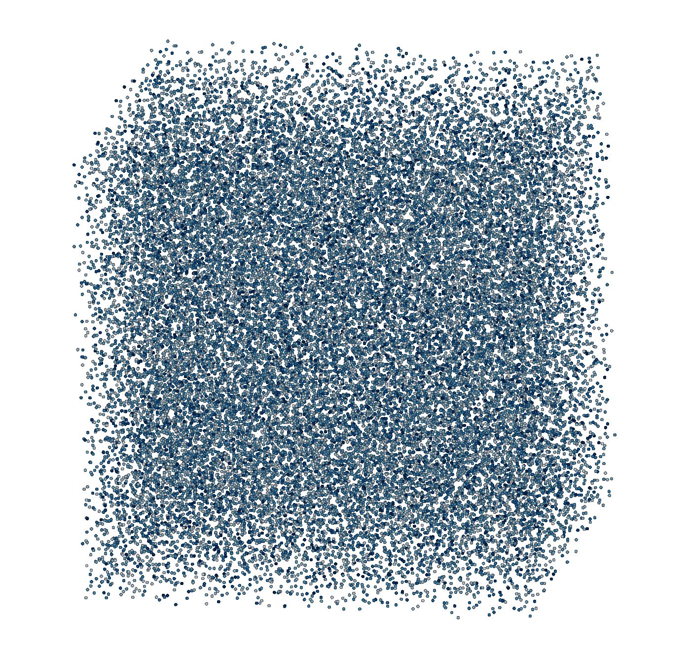
DPD solvent at rest
We will now run a simulation of particles in a periodic box interacting with Pairwise forces of type “DPD”.
We use a VelocityVerlet integrator to advance particles in time.
The initial conditions are Uniform randomly placed particles in the domain with a given density.
#!/usr/bin/env python

import mirheo as mir

dt = 0.001
rc = 1.0      # cutoff radius
number_density = 8.0

ranks  = (1, 1, 1)
domain = (16.0, 16.0, 16.0)

u = mir.Mirheo(ranks, domain, debug_level=3, log_filename='log')

pv = mir.ParticleVectors.ParticleVector('pv', mass = 1.0) # Create a simple Particle Vector (PV) named 'pv'
ic = mir.InitialConditions.Uniform(number_density)        # Specify uniform random initial conditions
u.registerParticleVector(pv, ic)                          # Register the PV and initialize its particles

# Create and register DPD interaction with specific parameters and cutoff radius
dpd = mir.Interactions.Pairwise('dpd', rc, kind="DPD", a=10.0, gamma=10.0, kBT=1.0, power=0.5)
u.registerInteraction(dpd)

# Tell the simulation that the particles of pv interact with dpd interaction
u.setInteraction(dpd, pv, pv)

# Create and register Velocity-Verlet integrator
vv = mir.Integrators.VelocityVerlet('vv')
u.registerIntegrator(vv)

# This integrator will be used to advance pv particles
u.setIntegrator(vv, pv)

# Write some simulation statistics on the screen every 500 time steps
u.registerPlugins(mir.Plugins.createStats('stats', every=500))

# Dump particle data
dump_every = 500
u.registerPlugins(mir.Plugins.createDumpParticles('part_dump', pv, dump_every, [], 'h5/solvent_particles-'))

u.run(5002, dt=dt)
This example demonstrates how to build a simulation:
- Create the
coordinator - Create the simulation objects (particle vectors, initial conditions…)
- Register the above objects into the
coordinator(seeregister*functions) - link the registered objects together in the
coordinator(seeset*functions)
The above script can be run as:
mpirun -np 2 python3 rest.py
Note
The rest.py script contains plugins of type Stats
and ParticleDumper,
which needs a postprocess rank additionally to the simulation rank in order to be active.
The simulation is then launched with 2 ranks.
The execution should output the stats.txt file as well as information output in the console.
Additionally, the particle positions and velocities are dumped in the h5 folder.
Adding Walls
We extend the previous example by introducing Walls in the simulation.
Two components are required to form walls:
- a geometry representation of the wall surface. In Mirheo, wall surfaces are represented as zero level set of a Signed Distance Function (SDF). This is used to decide which particles are kept at the beginning of the simulation, but also to prevent penetrability of the walls by solvent particles.
- frozen particles, a layer of particles outside of the wall geometry which interact with the inside particles to prevent density fluctuations in the vicinity of the walls.
Note
The user has to set the interactions with the frozen particles explicitly
#!/usr/bin/env python

import mirheo as mir

rc = 1.0      # cutoff radius
number_density = 8.0
dt = 0.001
ranks  = (1, 1, 1)
domain = (16.0, 16.0, 16.0)

u = mir.Mirheo(ranks, domain, debug_level=3, log_filename='log')

pv  = mir.ParticleVectors.ParticleVector('pv', mass = 1.0)
ic  = mir.InitialConditions.Uniform(number_density)
dpd = mir.Interactions.Pairwise('dpd', rc, kind="DPD", a=10.0, gamma=10.0, kBT=1.0, power=0.5)
vv  = mir.Integrators.VelocityVerlet('vv')

u.registerInteraction(dpd)
u.registerParticleVector(pv, ic)
u.registerIntegrator(vv)

# creation of the walls
# we create a cylindrical pipe passing through the center of the domain along
center = (domain[1]*0.5, domain[2]*0.5) # center in the (yz) plane
radius = 0.5 * domain[1] - rc           # radius needs to be smaller than half of the domain
                                        # because of the frozen particles

wall = mir.Walls.Cylinder("cylinder", center=center, radius=radius, axis="x", inside=True)

u.registerWall(wall) # register the wall in the coordinator

# we now create the frozen particles of the walls
# the following command is running a simulation of a solvent with given density equilibrating with dpd interactions and vv integrator
# for 1000 steps.
# It then selects the frozen particles according to the walls geometry, register and returns the newly created particle vector.
pv_frozen = u.makeFrozenWallParticles(pvName="wall", walls=[wall], interactions=[dpd], integrator=vv, number_density=number_density, dt=dt)

# set the wall for pv
# this is required for non-penetrability of the solvent thanks to bounce-back
# this will also remove the initial particles which are not inside the wall geometry
u.setWall(wall, pv)

# now the pv also interacts with the frozen particles!
u.setInteraction(dpd, pv, pv)
u.setInteraction(dpd, pv, pv_frozen)

# pv_frozen do not move, only pv needs an integrator in this case
u.setIntegrator(vv, pv)

u.registerPlugins(mir.Plugins.createStats('stats', every=500))
dump_every = 500
u.registerPlugins(mir.Plugins.createDumpParticles('part_dump', pv, dump_every, [], 'h5/solvent_particles-'))

# we can also dump the frozen particles for visualization purpose
u.registerPlugins(mir.Plugins.createDumpParticles('part_dump_wall', pv_frozen, dump_every, [], 'h5/wall_particles-'))

# we can dump the wall sdf in xdmf + h5 format for visualization purpose
# the dumped file is a grid with spacings h containing the SDF values
u.dumpWalls2XDMF([wall], h = (0.5, 0.5, 0.5), filename = 'h5/wall')

u.run(5002, dt=dt)
Note
A ParticleVector returned by makeFrozenWallParticles is automatically registered in the coordinator.
There is therefore no need to provide any InitialConditions object.
This example demonstrates how to construct walls:
- Create
Wallsrepresentation - Create
Interactionsand anIntegratorto equilibrate frozen particles - Create the frozen particles with
mmirheo.Mirheo.makeFrozenWallParticles() - Set walls to given PVs with
mmirheo.Mirheo.setWall() - Set interactions with the frozen particles as normal PVs
The execution of walls.py should output the stats.txt file as well as information output in the console.
Additionally, frozen and solvent particles, as well as the walls SDF are dumped in the h5 folder.
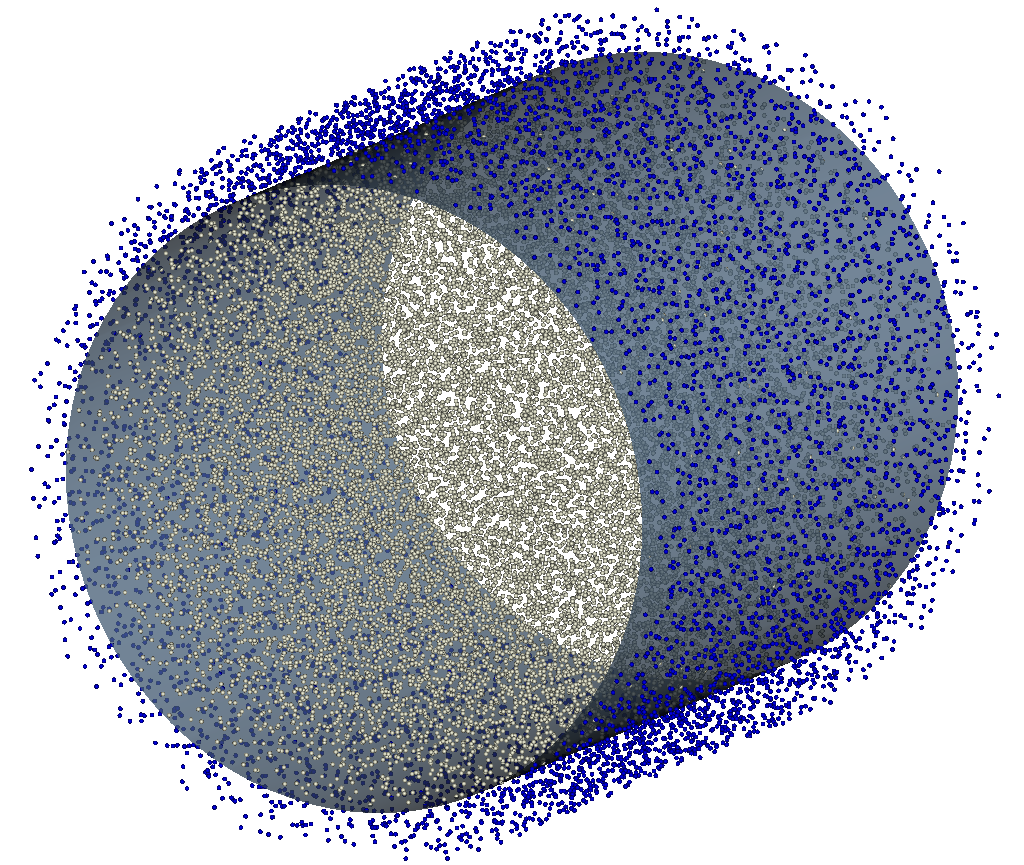
Snapshot of the data dumped by executing the walls.py script. The white particles represent the solvent, the blue particles are the frozen wall particles and the surface is the 0 level set of the SDF file.
Membranes
Membranes are a set of particles connected into a triangle mesh.
They can interact as normal PVs but have additional internal interactions, which we will use in this example.
Here we simulate one membrane with a given initial mesh “rbc_mesh.py” which can be taken from the data/ folder of the repository.
The membrane is subjected to shear, bending, viscous and constraint forces and evolves over time thanks to a VelocityVerlet integrator.
#!/usr/bin/env python

import mirheo as mir

dt = 0.001

ranks  = (1, 1, 1)
domain = (12, 12, 12)

u = mir.Mirheo(ranks, domain, debug_level=3, log_filename='log')

# we need to first create a mesh before initializing the membrane vector
mesh_rbc = mir.ParticleVectors.MembraneMesh("rbc_mesh.off")

# create a MembraneVector with the given mesh
pv_rbc   = mir.ParticleVectors.MembraneVector("rbc", mass=1.0, mesh=mesh_rbc)
# place initial membrane
# we need a position pos and an orientation described by a quaternion q
# here we create only one membrane at the center of the domain
pos_q = [0.5*domain[0], 0.5*domain[1], 0.5*domain[2], # position
         1.0, 0.0, 0.0, 0.0]                          # quaternion
ic_rbc   = mir.InitialConditions.Membrane([pos_q])
u.registerParticleVector(pv_rbc, ic_rbc)

# next we store the parameters in a dictionary
prms_rbc = {
    "x0"     : 0.457,
    "ka_tot" : 4900.0,
    "kv_tot" : 7500.0,
    "ka"     : 5000,
    "ks"     : 0.0444 / 0.000906667,
    "mpow"   : 2.0,
    "gammaC" : 52.0,
    "kBT"    : 0.0,
    "tot_area"   : 62.2242,
    "tot_volume" : 26.6649,
    "kb"     : 44.4444,
    "theta"  : 6.97
}

# now we create the internal interaction
# here we take the WLC model for shear forces and Kantor model for bending forces.
# the parameters are passed in a kwargs style
int_rbc = mir.Interactions.MembraneForces("int_rbc", "wlc", "Kantor", **prms_rbc)

# then we proceed as usual to make th membrane particles evolve in time
vv = mir.Integrators.VelocityVerlet('vv')
u.registerIntegrator(vv)
u.setIntegrator(vv, pv_rbc)
u.registerInteraction(int_rbc)
u.setInteraction(int_rbc, pv_rbc, pv_rbc)

# dump the mesh every 50 steps in ply format to the folder 'ply/'
u.registerPlugins(mir.Plugins.createDumpMesh("mesh_dump", pv_rbc, 50, "ply/"))

u.run(5002, dt=dt)
Note
The interactions handle different combinations of shear and bending models.
Each model may require different parameters.
Refer to mmirheo.Interactions.MembraneForces() for more information on the models and their corresponding parameters.
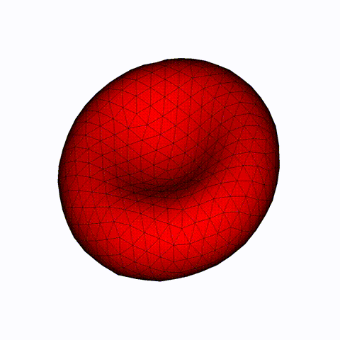
Sequence data dumped by executing the membrane.py script.
Creating Cells with Different inner and outer liquids
It is easy to extend the above simple examples into quite complicated simulation setups.
In this example we simulate a suspension of a few membranes inside a solvent.
We also show here how to split inside from outside solvents into 2 ParticleVectors.
This is useful when the 2 solvents do not have the same properties (such as viscosity).
The example also demonstrates how to avoid penetration of the solvents through the membranes thanks to mmirheo.Bouncers.
Note that in this example, we also show that it is easy to add many different interactions between given particle vectors.
#!/usr/bin/env python

import mirheo as mir

dt = 0.001
rc = 1.0
number_density = 8.0

ranks  = (1, 1, 1)
domain = (16.0, 16.0, 16.0)

u = mir.Mirheo(ranks, domain, debug_level=3, log_filename='log')

# create the particle vectors
#############################

# create MembraneVector for membranes
mesh_rbc = mir.ParticleVectors.MembraneMesh("rbc_mesh.off")

pv_rbc = mir.ParticleVectors.MembraneVector("rbc", mass=1.0, mesh=mesh_rbc)
pos_qs = [[ 5.0,  5.0, 2.0,     1.0, 0.0, 0.0, 0.0], # we create 4 membranes
          [11.0,  5.0, 6.0,     1.0, 0.0, 0.0, 0.0],
          [5.0,  11.0, 10.0,    1.0, 0.0, 0.0, 0.0],
          [11.0, 11.0, 14.0,    1.0, 0.0, 0.0, 0.0]]
ic_rbc   = mir.InitialConditions.Membrane(pos_qs)
u.registerParticleVector(pv_rbc, ic_rbc)

# create particleVector for outer solvent
pv_outer = mir.ParticleVectors.ParticleVector('pv_outer', mass = 1.0)
ic_outer = mir.InitialConditions.Uniform(number_density)
u.registerParticleVector(pv_outer, ic_outer)

# To create the inner solvent, we split the outer solvent (which originally occupies
# the whole domain) into outer and inner solvent
# This is done thanks to the belonging checker:
inner_checker = mir.BelongingCheckers.Mesh("inner_solvent_checker")

# the checker needs to be registered, as any other object; it is associated to a given object vector
u.registerObjectBelongingChecker(inner_checker, pv_rbc)

# we can now apply the checker to create the inner PV
pv_inner = u.applyObjectBelongingChecker(inner_checker, pv_outer, correct_every = 0, inside = "pv_inner")


# interactions
##############

prms_rbc = {
    "x0"     : 0.457,
    "ka_tot" : 4900.0,
    "kv_tot" : 7500.0,
    "ka"     : 5000,
    "ks"     : 0.0444 / 0.000906667,
    "mpow"   : 2.0,
    "gammaC" : 52.0,
    "kBT"    : 0.0,
    "tot_area"   : 62.2242,
    "tot_volume" : 26.6649,
    "kb"     : 44.4444,
    "theta"  : 6.97
}

int_rbc = mir.Interactions.MembraneForces("int_rbc", "wlc", "Kantor", **prms_rbc)
int_dpd_oo = mir.Interactions.Pairwise('dpd_oo', rc, kind="DPD", a=10.0, gamma=10.0, kBT=1.0, power=0.5)
int_dpd_ii = mir.Interactions.Pairwise('dpd_ii', rc, kind="DPD", a=10.0, gamma=20.0, kBT=1.0, power=0.5)
int_dpd_io = mir.Interactions.Pairwise('dpd_io', rc, kind="DPD", a=10.0, gamma=15.0, kBT=1.0, power=0.5)
int_dpd_sr = mir.Interactions.Pairwise('dpd_sr', rc, kind="DPD", a=0.0, gamma=15.0, kBT=1.0, power=0.5)

u.registerInteraction(int_rbc)
u.registerInteraction(int_dpd_oo)
u.registerInteraction(int_dpd_ii)
u.registerInteraction(int_dpd_io)
u.registerInteraction(int_dpd_sr)

u.setInteraction(int_dpd_oo, pv_outer, pv_outer)
u.setInteraction(int_dpd_ii, pv_inner, pv_inner)
u.setInteraction(int_dpd_io, pv_inner, pv_outer)

u.setInteraction(int_rbc, pv_rbc, pv_rbc)

u.setInteraction(int_dpd_sr, pv_outer, pv_rbc)
u.setInteraction(int_dpd_sr, pv_inner, pv_rbc)

# integrators
#############

vv = mir.Integrators.VelocityVerlet('vv')
u.registerIntegrator(vv)

u.setIntegrator(vv, pv_outer)
u.setIntegrator(vv, pv_inner)
u.setIntegrator(vv, pv_rbc)

# Bouncers
##########

# The solvent must not go through the membrane
# we can enforce this by setting a bouncer
bouncer = mir.Bouncers.Mesh("membrane_bounce", "bounce_maxwell", kBT=0.5)

# we register the bouncer object as any other object
u.registerBouncer(bouncer)

# now we can set what PVs bounce on what OV:
u.setBouncer(bouncer, pv_rbc, pv_outer)
u.setBouncer(bouncer, pv_rbc, pv_inner)

# plugins
#########

u.registerPlugins(mir.Plugins.createStats('stats', every=500))

dump_every = 500
u.registerPlugins(mir.Plugins.createDumpParticles('part_dump_inner', pv_inner, dump_every, [], 'h5/inner-'))
u.registerPlugins(mir.Plugins.createDumpParticles('part_dump_outer', pv_outer, dump_every, [], 'h5/outer-'))
u.registerPlugins(mir.Plugins.createDumpMesh("mesh_dump", pv_rbc, dump_every, "ply/"))

u.run(5002, dt=dt)
Note
A ParticleVector returned by applyObjectBelongingChecker is automatically registered in the coordinator.
There is therefore no need to provide any InitialConditions object.
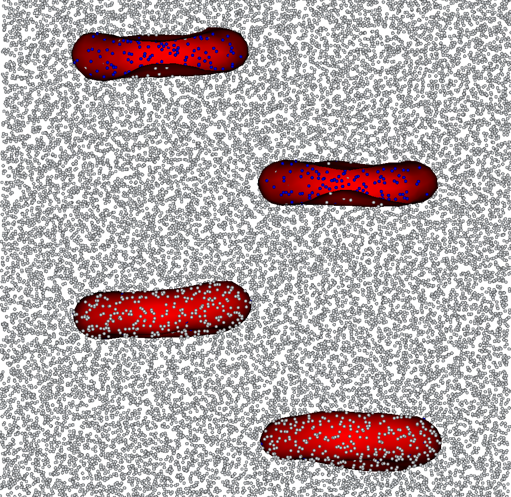
Snapshots of the output files from membranes_solvents.py. White particles are the outer solvent, blue particles are inner. Two of the four membranes are cut for visualization purpose.
Creating Rigid Objects
Rigid objects are modeled as frozen particles moving together in a rigid motion, together with bounce back of particles, similarly to the walls.
In Mirheo, we need to create a RigidObjectVector, in which each rigid object has the same frozen particles template.
Generating these frozen particles can be done in a separate simulation using a BelongingChecker.
This is shown in the following script for the simple mesh sphere_mesh.off which can be found in the data/ folder:
import mirheo as mir
import numpy as np
import trimesh

def recenter(coords, com):
    coords = [[r[0]-com[0], r[1]-com[1], r[2]-com[2]] for r in coords]
    return coords

dt = 0.001
rc = 1.0
mass = 1.0
number_density = 10.0
niter = 1000

# the triangle mesh used to create the object
# here we load the file using trimesh for convenience
m = trimesh.load("sphere_mesh.off");

# trimesh is able to compute the inertia tensor
# we assume it is diagonal here
inertia = [row[i] for i, row in enumerate(m.moment_inertia)]

ranks  = (1, 1, 1)
domain = (16, 16, 16)

u = mir.Mirheo(ranks, domain, debug_level=3, log_filename='log')

dpd = mir.Interactions.Pairwise('dpd', rc, kind="DPD", a=10.0, gamma=10.0, kBT=0.5, power=0.5)
vv  = mir.Integrators.VelocityVerlet('vv')

# we create here a fake rigid object in the center of the domain with only 2 particles
# those particles will be used to compute the extents in the object belonging, so they
# must be located in the to corners of the bounding box of the object
# this is only to be able to make use of the belonging checker

bb_hi = m.vertices.max(axis=0).tolist()
bb_lo = m.vertices.min(axis=0).tolist()

coords = [bb_lo, bb_hi]
com_q = [[0.5 * domain[0], 0.5 * domain[1], 0.5 * domain[2],   1, 0, 0, 0]]

mesh = mir.ParticleVectors.Mesh(m.vertices.tolist(), m.faces.tolist())
fake_ov = mir.ParticleVectors.RigidObjectVector('fake_ov', mass, inertia, len(coords), mesh)
fake_ic = mir.InitialConditions.Rigid(com_q, coords)

belonging_checker = mir.BelongingCheckers.Mesh("mesh_checker")

# similarly to wall creation, we freeze particles inside a rigid object
pv_rigid = u.makeFrozenRigidParticles(belonging_checker, fake_ov, fake_ic, [dpd], vv, number_density, mass, dt=dt, nsteps=niter)

if u.isMasterTask():
    coords = pv_rigid.getCoordinates()
    coords = recenter(coords, com_q[0])
    np.savetxt("rigid_coords.txt", coords)
Note
here we make use of trimesh as we need some properties of the mesh. This would also allow to load many other formats not supported by Mirheo, such as ply.
Note
The saved coordinates must be in the frame of reference of the rigid object, hence the shift at the end of the script.
We can now run a simulation using our newly created rigid object. Let us build a suspension of spheres in a DPD solvent:
#!/usr/bin/env python

import mirheo as mir
import numpy as np
import trimesh

dt = 0.001
rc = 1.0
mass = 1.0
number_density = 10

m = trimesh.load("sphere_mesh.off");
inertia = [row[i] for i, row in enumerate(m.moment_inertia)]

ranks  = (1, 1, 1)
domain = (16, 8, 8)

u = mir.Mirheo(ranks, domain, debug_level=3, log_filename='log', no_splash=True)

pv_solvent = mir.ParticleVectors.ParticleVector('solvent', mass)
ic_solvent = mir.InitialConditions.Uniform(number_density)

dpd = mir.Interactions.Pairwise('dpd', rc, kind="DPD", a=10.0, gamma=10.0, kBT=0.01, power=0.5)
# repulsive LJ to avoid overlap between spheres
cnt = mir.Interactions.Pairwise('cnt', rc, kind="RepulsiveLJ", epsilon=0.28, sigma=0.8, max_force=400.0)

vv = mir.Integrators.VelocityVerlet_withPeriodicForce('vv', force=1.0, direction="x")

com_q = [[2.0, 6.0, 5.0,   1.0, 0.0, 0.0, 0.0],
         [6.0, 7.0, 5.0,   1.0, 0.0, 0.0, 0.0],
         [10., 6.0, 5.0,   1.0, 0.0, 0.0, 0.0],
         [4.0, 2.0, 4.0,   1.0, 0.0, 0.0, 0.0],
         [8.0, 3.0, 2.0,   1.0, 0.0, 0.0, 0.0]]

coords = np.loadtxt("rigid_coords.txt").tolist()
mesh = mir.ParticleVectors.Mesh(m.vertices.tolist(), m.faces.tolist())

pv_rigid = mir.ParticleVectors.RigidObjectVector('spheres', mass, inertia, len(coords), mesh)
ic_rigid = mir.InitialConditions.Rigid(com_q, coords)
vv_rigid = mir.Integrators.RigidVelocityVerlet("vv_rigid")

u.registerParticleVector(pv_solvent, ic_solvent)
u.registerIntegrator(vv)
u.setIntegrator(vv, pv_solvent)

u.registerParticleVector(pv_rigid, ic_rigid)
u.registerIntegrator(vv_rigid)
u.setIntegrator(vv_rigid, pv_rigid)

u.registerInteraction(dpd)
u.registerInteraction(cnt)
u.setInteraction(dpd, pv_solvent, pv_solvent)
u.setInteraction(dpd, pv_solvent, pv_rigid)
u.setInteraction(cnt, pv_rigid, pv_rigid)

# we need to remove the solvent particles inside the rigid objects
belonging_checker = mir.BelongingCheckers.Mesh("mesh checker")
u.registerObjectBelongingChecker(belonging_checker, pv_rigid)
u.applyObjectBelongingChecker(belonging_checker, pv_solvent, correct_every=0, inside="none", outside="")

# apply bounce
bb = mir.Bouncers.Mesh("bounce_rigid", "bounce_maxwell", kBT=0.01)
u.registerBouncer(bb)
u.setBouncer(bb, pv_rigid, pv_solvent)

# dump the mesh every 200 steps in ply format to the folder 'ply/'
u.registerPlugins(mir.Plugins.createDumpMesh("mesh_dump", pv_rigid, 200, "ply/"))

u.run(10000, dt=dt)
Note
We again used a BelongingChecker in order to remove the solvent inside the rigid objects.
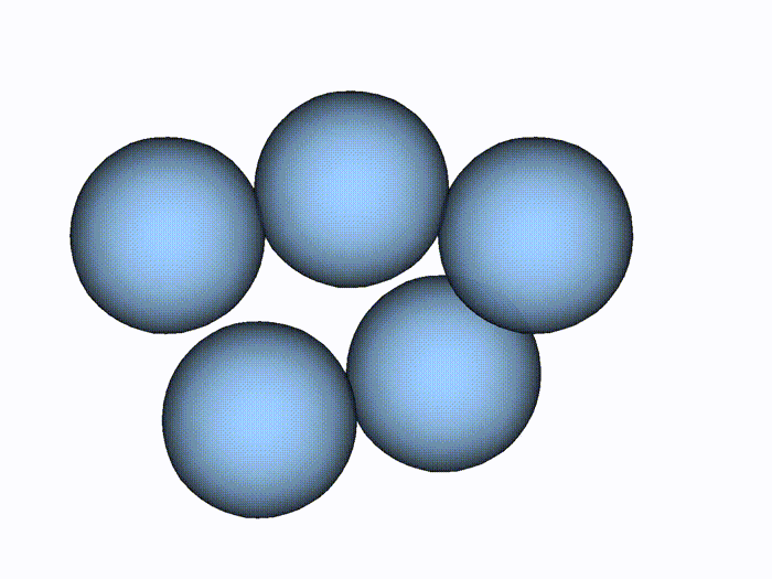
Snapshots of the output files from rigid_suspension.py.